1 Data
For the purpose of modeling the impacts of environmental change, several data sets were used which are described in the chapters below. To establish a water model for selected catchments, these data were observed data (Chapter 1.1). This data set was also used in generating the climate change scenarios based on simulations performed under the projects called ENSEMBLES (Chapter 1.2) and CMIP5 (Chapter 1.3).
1.1 Observed data and selection of the set of catchments
For the purpose of assessing the changes to the water balance, a total of 130 catchments and intercatchments more or less encompassing the Czech Republic territory (see Fig. 1.1). The definitions of the various catchments can be found in Annex P.1. Our selection was based on third-order catchments. Depending on availability of the observed series the catchment and intercatchment boundaries were optimized so as to obtain units of interest having areas of approximately the same size and to have observed runoff data available for calibrating the hydrological model called Bilan. In computing the intercatchment runoffs in particular, where the amount of runoff is derived from the differences in runoff of the partial catchments involved, the availability of data imposed a considerable limitation (more on this in Chapter 2).
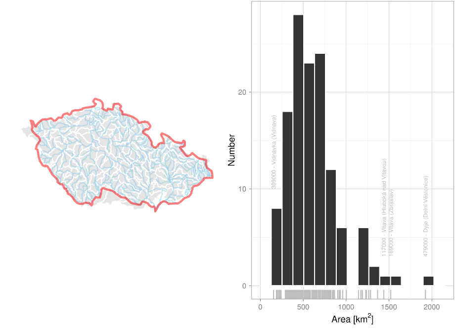
Fig.1.1 Selected set of catchments (left) and their geographic areas (right).
For the purpose of calibrating the Bilan hydrological model, the monthly precipitation and temperature time series for the 1961–2010 period were used in addition to the monthly runoff series. These series were derived from gridded precipitation and temperature datasets having a resolution of 25 km × 25 km (Štěpánek et al. 2011). For the catchments under scrutiny, interpolation using Thiessen polygons yielded the average precipitation values per catchment, which were subsequently corrected based on the average precipitation depth (the same period, resolution 1 km × 1 km) so as to result in the same average precipitation for all the catchments. Temperature corrections were applied in an analogous way – the average temperature for the catchment determined from the gridded depth was corrected based on the differences in altitude above sea level derived from the gridded depth and from a digital ground model, assuming a temperature gradient of 0.65 °C/100 m. The daily gridded dataset was also employed to generate the climate change scenarios using a correction for systematic error (see Chapter 4.1) and an advanced incremental algorithm (see Chapter 4.2).
1.2 Regional climate models from the ENSEMBLES project
The ENSEMBLES project (Hewitt a Griggs 2004) was a major project funded from EU FP7, participated by dozens of mainly European institutions. A number of simulations of global and regional climate models were performed under this project, mostly for Europe but also for West Africa. Simulations of regional climate models are available in the form of 40-year time sections controlled by ERA-40 reanalysis on the one hand and of so-called transient simulations controlled by global climate models on the other hand, for the 1950–2050 or even the 1950–2100 period. The regional climate model data can be downloaded from http://ensemblesrt3.dmi.dk/.
This project made use of simulations controlled by the SRES A1B emission scenario (other emission scenarios being rather scarce in the ENSEMBLES data), which covers the 1961-2099 period with a spatial resolution of 25 km × 25 km. A total of 15 RCM simulations controlled by 4 GCM models were considered (see Table 1.1). The greatest number of simulations (4) was run using the RCA model. Within this set of models, a special position is enjoyed by the HadRM simulations which involve three members of the so-called perturbed physics ensemble – i.e., a file produced by a systematic alteration of the parameters of the HadRM model. The HadRM_Q0 model has standard settings, the HadRM_Q3 (HadRM_Q16) model as the lowest (highest) response to radiation effects (see Collins et al. 2006)
Table 1.1. The regional climate model simulations performed
| Model | Acronym | Source |
|---|---|---|
| controled by model ECHAM5 | ||
| RACMO | RACMO_EH5 | Royal Netherlands Meteorological Institute (KNMI) |
| REMO | REMO_EH5 | Max-Planck Institut (MPI), Germany |
| RCA | RCA_EH5 | Swedish Hydrometeorological Institute (SMHI) |
| RegCM | RegCM_EH5 | International Centre for Theoretical Physics (ICTP), Italy |
| HIRHAM | HIR_EH5 | Danish Meteorological Institute (DMI) |
| controled by model HadCM3Q0, HadCM3Q3, HadCM3Q16 | ||
| HadRM | HadRM_Q0 | Hadley Centre, UK |
| CLM | CLM_Q0 | Swiss Federal Institute of Technology (ETHZ) |
| HadRM | HadRM_Q3 | Hadley Centre, UK |
| RCA | RCA_Q3 | Swedish Hydrometeorological Institute (SMHI) |
| HadRM | HadRM_Q16 | Hadley Centre, UK |
| RCA | RCA_Q16 | Community Alliance for Climate Change (C4I), Ireland |
| controled by model ARPEGE | ||
| HIRHAM | HIR_ARP | Danish Meteorological Institute (DMI) |
| CNRM-RM | CNRM_ARP | National Centre for Meteorological Research (CNRM), France |
| ALADIN-CLIMATE/CZ* | ALA_ARP | Czech Hydrometeorological Institute (ČHMÚ), Czech Republic |
| controled by model BCM | ||
| RCA | RCA_BCM | Swedish Hydrometeorological Institute (SMHI) |
*)This simulation was produced under an R&D project called ‘More accurate estimates of climate change impacts as observed within the provinces of water management, agriculture and forestry, and the adaptative measures proposed’
1.3 Global climate models from the CMIP5 project
The Coupled Model Intercomparison Project (CMIP), which now has reached its fifth phase (i.e., CMIP5) was launched in 2008 aiming mainly to establish a framework for the coordination of climate modeling experiments, with a special focus on the IPCC Fifth assessment report (Stocker et al. 2013). The declared objective of the project is to provide a multi-model context that would serve (1) to evaluate the mechanisms responsible for the differences in feedback simulations connected primarily with the carbon cycle and with cloud formation, (2) to verify the climate prediction capability of the models on the scale of decades, and (3) to identify the reasons for the differences in projections generated by models having the same type of control.
The CMIP5 models make use (inter alia) of the RCP concentrations scenario. The entire set of models is unique in terms of size – at the stage of data acquisition for this study the available body of data included data from 30 GCMs from 18 institutions, totaling 191 simulations (see Table 1.2). The various RCP scenarios are not uniformly represented – there are 63 and only 29 simulations available for RCP8.5 and RCP6.0, respectively. For some GCMs there are several simulations available for a given RCP scenario (the maximum is 10 for CSIRO-Mk3-6-0), but most of the models have only one simulation for any given RCP scenario. Moreover, not all the models are so adapted as to produce simulations for all RCP scenarios.
Available data included daily GCM data interpolated on a common 1.25° × 2° grid for the periods 1961–1995, 2021–2050, and 2071–2100.
Table 1.2. Number of simulations available for all GCM and RCP combinations employed (MODEL: global model identifier, ACM: atmospheric model identifier)
| MODEL | ACM | RCP | \(\mathbf{\sum}\) | MODEL | ACM | RCP | \(\mathbf{\sum}\) | ||||||
|---|---|---|---|---|---|---|---|---|---|---|---|---|---|
| 2.6 | 4.5 | 6.0 | 8.5 | 2.6 | 4.5 | 6 | 8.8 | ||||||
| CNRM-CM5 | ARPEGE | 1 | 1 | - | 1 | 3 | GFLD-CM3 | GFLD | 1 | - | 1 | 1 | 3 |
| EC-EARTH | - | - | - | 8 | 8 | GFDL-ESM2G | 1 | 1 | 1 | 1 | 4 | ||
| bcc-csm1-1 | BCC | 1 | 1 | 1 | 1 | 4 | GFDL-ESM2M | 1 | 1 | 1 | 1 | 4 | |
| bcc-csm1-1-m | 1 | 1 | 1 | 1 | 4 | GISS-E2-R | GISS | - | 1 | - | - | 1 | |
| MRI-CGCM3 | MRI | 1 | 1 | 1 | 1 | 4 | ACCESS1-3 | GA | - | 1 | - | 1 | 2 |
| BNU-ESM | CAM | 1 | 1 | - | 1 | 3 | ACCESS1-4 | HadGEM | - | 1 | - | 1 | 2 |
| CCSM4 | 3 | 3 | 3 | 3 | 12 | HadGEM-CC | - | 1 | - | 3 | 4 | ||
| NorESM1-M | 1 | 1 | 1 | 1 | 4 | HadGEM2-ES | 4 | 4 | 4 | 4 | 16 | ||
| CanESM2 | CanCM | 5 | 5 | - | 5 | 15 | inmcm4 | INCM | - | 1 | - | 1 | 2 |
| CSIRO-Mk3-6-0 | CSIRO | 10 | 10 | 10 | 10 | 40 | IPSL-CM5A-LR | IPSL | 4 | 4 | 1 | 4 | 13 |
| CMCC-CESM | ECHAM | - | - | - | 1 | 1 | IPSL-CM5A-MR | 1 | 1 | 1 | 1 | 4 | |
| CMCC-CM | - | 1 | - | 1 | 2 | IPSL-CM5B-LR | IPSL-B | - | 1 | - | 1 | 2 | |
| CMCC-CMS | - | 1 | - | 1 | 2 | MIROC5 | MIROC | 3 | 3 | 1 | 3 | 10 | |
| MPI-ESM-LR | 3 | 3 | - | 3 | 9 | MIROC-ESM | 1 | 1 | 1 | 1 | 4 | ||
| MPI-ESM-MR | 1 | 3 | - | 1 | 5 | MIROC-ESM-CHEM | 1 | 1 | 1 | 1 | 4 | ||
| \(\mathbf{\sum}\) | 45 | 54 | 29 | 63 | 191 |
2 The Bilan hydrological model and its calibration
The Bilan hydrological model (Horáček et al. 2009) offers a schematic representation of the catchment by a system of reservoirs situated at three elevations – the ground i.e. the surface of terrain, the soil zone, and the groundwater zone. The amount of flow in-between the individual reservoirs is determined by the model algorithms, controlled by eight and six free parameters in its monthly and daily versions, respectively (see Table 2.1). The observed precipitation and air temperature time series are the model inputs. Potential evapotranspiration is computed by a simple method (Oudin et al. 2010; Beran et al. 2011) based on air temperature and solar radiation incident on the upper layer of the atmosphere (influenced by latitude and the day of the year), os as the case may be, by a method (Gidrometeoizdat, 1976) based on empirical relationships (derived for various vegetation zones) between potential evapotranspiration and the saturation complement computed from air temperature and relative humidity. The balance on the soil surface is determined by the precipitation totals at input and by the basin evaporation determined on the basis of potential evapotranspiration and the quantity of water available. In wintertime and during the thaw, the surface balance is influenced by the value of snow water storage. Water infiltrates from the surface into the soil zone where it fills the reservoir to a capacity which is one of the calibrated parameters. On overstepping this capacity, water is drained away and, subsequently, is split between two linear reservoirs. Their runoffs represent the slow (baseflow) and rapid (direct runoff) response of the catchment, while the value of total runoff is the sum of the two (Horáček et al. 2009).
Table 2.1. Parameters of the Bilan model
| Parameter | Meaning |
|---|---|
| Spa | capacity of soil moisture storage |
| Alfa | parameter of rainfall-runoff relationship between direct runoff and rainfall |
| Grd | parameter controlling outflow from groundwater storage (base flow) |
| Dgm | parameter expressing the rate of snowmelt dependably on the air temperature |
| Dgw | parameter for calculating the quantity of liquid water available on the land surface under winter conditions |
| Wic, Mec, Soc | parameter controlling outflow from groundwater storage (base flow) |
For the purpose of calibration of the Bilan model, tha available monthly time series of observed precipitation and temperature were compiled for the areas of 130 of these catchments chosen, for the 1961–2010 period. Further, the runoff series were derived for the closure profiles of the various catchments. The available time series of monitoring of the values of flow cover 68 catchments for the entire period under scrutiny, and 98, 109, 118, and 124 catchments for periods of at least 40 years, 30 years, 20 years, and 10 years, respectively. No serviceable data were available for four catchments (DBCN 153200, 169000, 205000, 480500). Some of these catchments are sections of streams rather than enclosed catchments in all cases, and this is why the computation of flow often is problematic – owing to inaccuracies and measuring errors the resultant flows based on the flow readings come out negative for the individual partial catchments in some months. For 88 catchments the series did not show any negative flow values, for 115 catchments the shares of negative flow values was 10% (Fig. 2.1). The number of years for which serviceable data exist and the ratios of negative flow values are can be found in the map shown on Fig. 2.2.
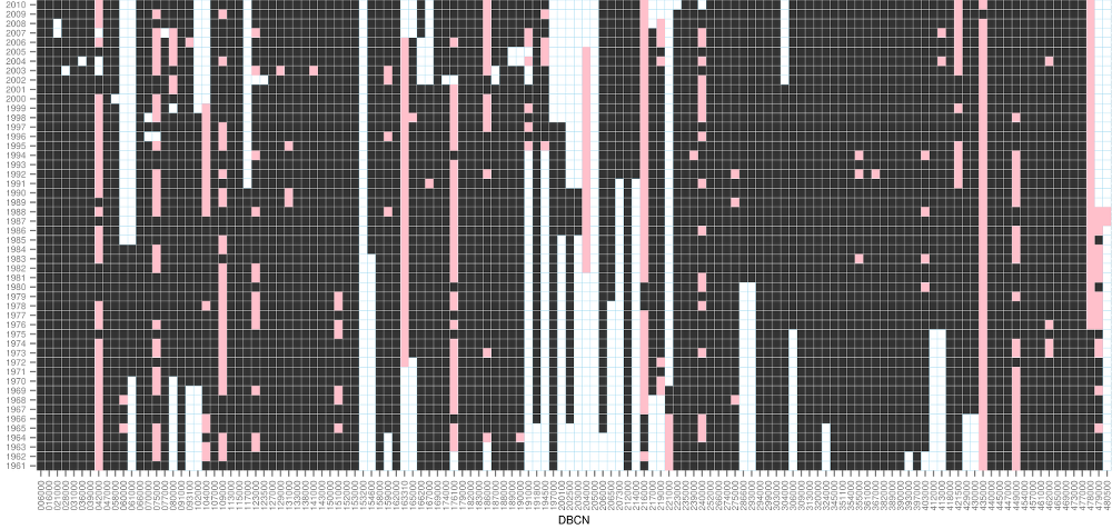
Fig. 2.1 Data overview. Years for which serviceable adata are available are shown in black; years exhibiting negative flow values are in pink; years for which no data are available are in white.
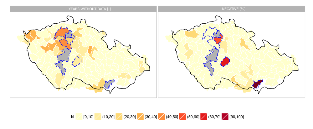
Fig. 2.2 The number of years for which there are no data during the 1961–2010 period (left) and the ratio of negative flow values (right). Those catchments for which no serviceable data were found are shown in gray. Those catchments for which the series of serviceable data are less than 10 years or for which the ratio of negative values is higher than 25 % are delineated in blue.
The reason of incidence of negative values in individual cases and of a systematic error in deriving the runoff from intercatchments in general may in part be due to the time step in-between the profiles and possibly also the water use. However, a large share of the systematic error may be attributed to the inaccuracy of flow measurements conducted in the profiles for which readings were taken. A detailed analysis of these errors under simplifying assumptions has been proposed (Kašpárek 1989). Let \(Q_d\) be the flow in the lower profile; the upper profile flow is a K-multiple of the lower one and thus, \(Q_h = K Q_d\) and the relative error of measurement, \(r\) is the same for both profiles. It cannot be said with any certainty how the partial errors \(r Q_h\) and \(r Q_d\) would either add together or partially compensate in any specific case. The total error may be derived using the sum of squares for error, i.e., \(e_r = \sqrt{(r Q_h)^2+(r Q_d)^2} = r Q_d \sqrt{1 + K^2}\) however, an more unfavorable case may also occur where the errors would add together, i.e., \(e^*_r = r (Q_h + Q_d) = r Q_d (1 + K)\)*. Rewriting these expressions it holds that for the relative runoff error we arrive at the expression
\[e_r = \frac{r \sqrt{1+ K^2}}{1-K},\](2.1)
or, for the more unfavorable case,
\[e_r^* = \frac{r (1+K)}{1-K}.\](2.2)
The coefficient \(K\) can be derived from the series of flow data, but these are themselves affected by the analyzed systematic error. Another option would be to make use of a hydrological analogy, i.e., to derive the coefficient \(K\) from the ratio of surface areas of the partial catchments. The coefficient \(K\) thus derived as well as the catchment categorisation into three classes by size are shown in Fig. 2.3. It is evident that in some cases, the error of estimate of the intercatchment runoff can be enormous. This can happen especially in the case of large-sized catchments for which the ratio of the intercatchment surface area (roughly comparable i.e., of the same order of magnitude for the 130 catchments selected) to the area of the remaining catchments is small.

Fig. 2.3 Relative error of estimate trends for the runoff from intercatchments, for different values of the error of measurement – \(e_r\) in solid line, \(e_r^*\) in dashed line (left), coefficient \(K\) from the equations – derived from the surface area difference (center) and the relative error of estimate of intercatchment runoff for a measuring error of 10 % (right).
Calibration was performed using the Bilan model routines, i.e., the parameters were optimized by the gradient method or by the differential evolution method (Máca et al. 2013). Both these methods allow for a selection of the optimization criterion out of the criteria which are used as standard in calibrating the hydrological models (Nash-Sutcliffe – NSE, log NSE, the mean square error – RMSE, the mean absolute error – MAE, the mean relative error – MAPE). In view of the incidence of negative values the optimization algorithm of the Bilan model has been adapted so as to allow weighting to be assigned to individual observation readings; in calibration, these weights are used to calculated the optimization criterion. Thus, by allocating zero or negative weights the effect of negative values on the value of the optimization criterion or on the resultant parameters can be entirely eliminated. Also, the option of performing the calibration taking the base flow estimate into account has been resorted to for a number of catchments. A base flow estimate obtained by the rolling minima method has been furnished by the Czech Hydrometeorological Institute.
Various optimization techniques, criterial functions, calibration periods etc. were tested for each catchment. For catchments where no reliable data were available, parameter sets transferred from nearby catchments were used. In a number of cases (owing to the nature of the data), calibration proceeded based on expert estimates rather than on a strict minimization/maximization of the pptimization criterion. At the first glance the results of calibration as expressed by the criterial function values are not entirely satisfactory. Nevertheless, taking into account the categorization of the catchments by the estimated error of runoff from the intercatchment (see Fig. 2.4), we find that those catchments which are burdened with smaller errors of runoff estimates also exhibit acceptable values of the criterial functions. On the contrary, in the case of catchments for which the data are unreliable the criteria indicate discrepancies between the estimated and simulated values. Hence the unsatisfactory values of the criterial functions can at least in part be ascribed to errors in determining the flows.
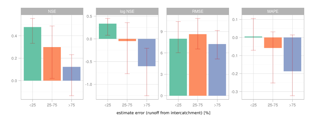
Fig. 2.4 Bar chart indicating the criterial function medians for various categories of reliability of estimates of intercatchment runoff. The lines in the graph indicate the interquartile span the catchments in the given category.
Owing to the difficulties of calibration we have focused on the validation of the simulated runoff values using empirical relations and on an analysis of the resultant parameters. In the first step the resultant parameter sets for the catchment were revised in cases where some of the parameters assumed values out of the ordinary (as a rule, values near one of the boundaries of the intervals used for calibrating the individual parameters).
Subsequently, an evaluation was made for the individual catchments to ascertain whether the simulated total runoff and base flow are consistent with the empirical estimates as presented e.g., by Kašpárek et al. (2012). The empirical relations considered were estimated from several data series encompassing dozens of catchments. It would of course be possible to directly include these relations in the Bilan model optimization, but this would only result in an artifical confirmation of those relations.
For catchments with annual average precipitation values (\(P_a\)) higher than 400 mm the annual average runoff height (\(R_a\)) can be determined by
\[R_a = 0.000571P^2_a + 0.132P_a - 170.2\](2.3)
An alternative has been proposed by Kašpárek et al. (2000) in the form
\[R_a = P_a + 0.519P^{1.236}_a - 2.967P_a - 98.1\](2.4)
The aforementioned formulas suffer from the drawback that, from the physical viewpoint, they entirely ignore the efect of temperature on evaporation and, therefore, also on the runoff value. Kašpárek et al. (2012) proposed the application of empirical relations to estimate the average annual potential evapotranspiration (\(PE_a\)) based on the average annual temperature (\(T_a\))
\[PE_a = 37.97 T_a + 289.4\](2.5)
as well as a relation giving the ratio of actually evapotranspired water (\(E_a\)) to potential evotranspiration
\[{\frac{E_a}{PE_a}} = 0.98 (1 - 0.22 ^ {\frac{P_a}{PE_a}}).\](2.6)
Using the hydrological balance \(R_a = P_a - E_a\) these relations can be used to express \(R_a\) as
\[R_a = P_a - 0.98 PE_a (1 - 0.22 ^ {\frac{P_a}{PE_a}}).\](2.7)
An empirical relation for the average base flow (\(q_z\) [l/s/km²]) was derived by Krásný et al. (1982) for catchments having no major natural sources:
\[q_z = 0.00001924 P_a^2 - 0.01251257 P_a + 2.06052230.\](2.8)
Based on the project Rebalance of underground water reserves, Beran et al. (2014) derived a relationship for the average annual base flow (\(BF\) [mm/rok])
\[BF = 0.0004 P_a^2 - 0.0276 P_a - 56.978.\](2.9)
In analogy to the equiations 2.3 and 2.4, the effect of temperature is not considered here.
A comparison of the total runoff and base flow based on the model with the empirical estimates is illustrated in Fig. 2.5. The total model runoff corresponds well with the empirical estimates. The base flow as per the Bilan model is somewhat biased compared to the empirical estimates (ca. −15% when using the formula by Krásný et al. (1982), and ca. +13% when using that by Beran et al. (2014)). Owing to the inaccuracies of measurement and errors of base flow estimates, the simulated values can be regarded as acceptable in either case.
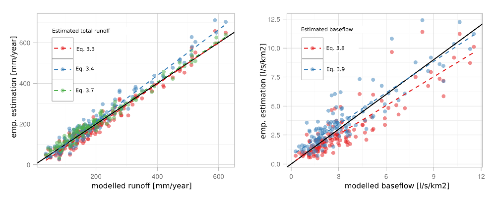
Fig. 2.5 Comparison of model total runoff (left) and base flow (right) with empirical formulas. The dashed line shows the linear model fit.
Eventually, the calibrated parameters were used for several types of simulation:
- Simulation for the conditions oberved based on a homogeneous gridded data series of precipitation and temperature covering the 1961–2010 period (see Chapter 3).
- Simulation for the climate change scenarios as per the corrected simulations of regional climate models from the ENSEMBLES project (see Chapter 4.1)
- Simulation for the climate change scenarios as per the corrected simulations of regional climate models from the CMIP5 project (see Chapter 4.2).
In the global perspective, this gives a true picture of the important features of the hydrological conditions prevailing in the Czech Republic. In individual cases the resultant parameters and the long-term averages of the simulated quantities need not be optimal. Efforts are being made to rectify these imperfections. Therefore, the results presented further on are also best suited for interpretation rather just on a regional scale within the Czech Republic, or at the catchment level.
3 The changes underway
Climate changes impacting Czech Republic’s hydrological conditions have been observed for a number of years already. The most distinctly marked of all these changes are the changes in air temperatures. Interpolating the air temperatures on the catchment areas we find that from the 1961–1990 period to the 1980–2010 period the average annual temperature hs risen 0.6°C and as much as 0.9°C in summertime, while in the fall the rise has been only 0.2°C (see Fig. 3.1). As to their spatial distribution, these temperature changes have been relative homogeneous – the catchment-to-catchment temperature rise difference for the various seasons of the year has been mostly no higher than 0.5°C, whereas the difference in the changes for different seasons has been as high as 1°C for some catchments.
Temperature is the principial factor impacting the hydrological balance, mainly for the reason that with rising temperature the quantity of water available for evaporation or, as the case may be, for transpiration by vegetation is growing, i.e., potential evaporanspiration increases with rising temperature. In analogy with temperature, the changes in potential evapotranspiration exhibit a homogeneous spatial distribution and reach 5% on the average throughout the seasons, the greatest change occurring in wintertime (10 %) due to a higher number of days with temperatures permitting evaporation, as opposed to the fall (1 % – compare with the temperature changes). Converted to the heights of the water column these changes correspond to approximately 25 mm for the whole year, of which the greatest change (13 mm) occurs in the summer and the smallest change (1 mm) in the fall. In spite of a high relative increase in potential evapotranspiration in wintertime the absolute change occurring in this season is also very small (1.5 mm).
In fact however the changes in evapotranspiration are smaller due to the fact that there is not enough water for evaporation and for transporation by the vegetation. Thus the actual evapotranspiration (Fig. 3.2) increases 3 % on the average (i.e., 11 mm per annum) and it is only during wintertime that this increase is roughly equal to potential evapotranspiration. During all the other seasons of the year the changes vary within units of percent; in sprintime and summertime this corresponds to ca. 5 mm.
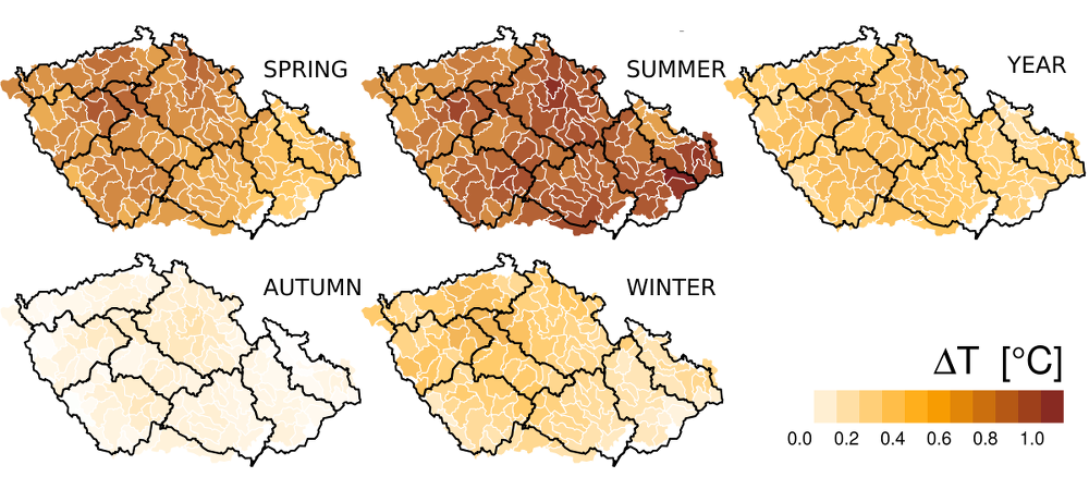
Fig. 3.1 Temperature changes from the 1961–1990 period to the 1980–2010 period for different seasons of the year.
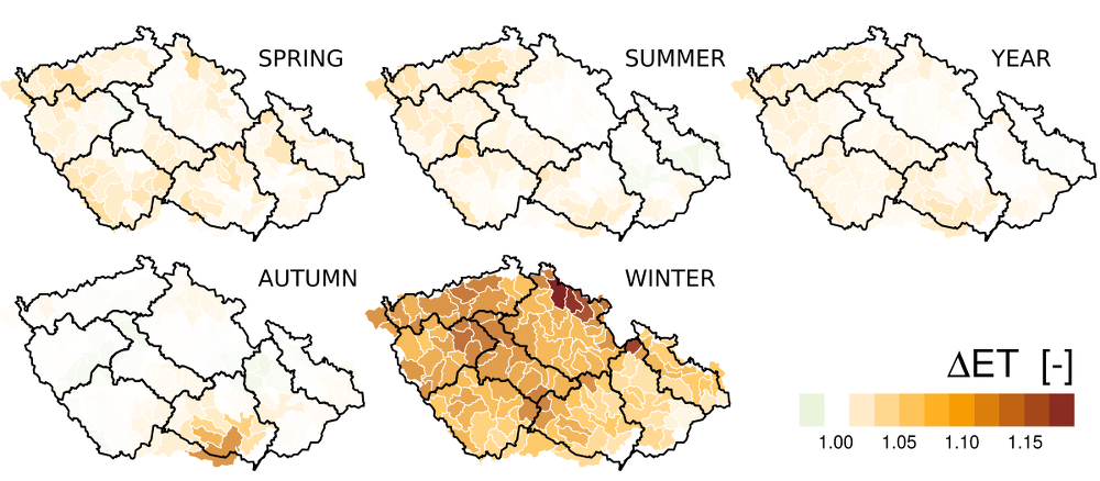
Fig. 3.2 Actual evapotranspiration changes (based on hydrological model estimates) from the 1961–1990 period to the 1980–2010 period for different seasons of the year.
It is a favorable circumstance for the hydrological conditions that the observed increase in temperature and in potential as well as actual evapotranspiration is accompanied by a moderate growth in precipitation (Fig. 3.3). The annual average total precipitation rose 3% (23 mm) from the 1961–1990 period to the 1981–2010 period, stagnated during springtime, and kept increasing approximately 5% (ca. 7 mm) during the other seasons. Unlike the temperature and evapotranspiration changes the changes observed in precipitation show considerable fluctuations in their spatial distribution. The territory of Central Bohemia is especially noteworthy: a decrease of springtime precipitation totals (of up to 10%) has been noted there. This decrease is also co-responsible for the stagnation of otherwise increasing annual precipitation totals for this region. This hegerogeneity may be partly explained by long-term changes in atmospheric circulation. The differences in the precipitation changes from one catchment to another have been 20% max. for all seasons of the years. This is roughly the same as the maximum seasonal precipitation change differences for the various catchments.
In the annual balance, on a great part of our territory there occurs an effective compensation of the growth of potential evapotranspiration by increased precipitation. Thus on the average there is a moderate increase of the annual runoff levels (ca. 4 %, 10 mm), see Fig. 3.4. This increase however is not of a wide-area nature – it is only on one quarter of the catchments under scrutiny that a decrease in runoff has been encountered (on nearly one half during summertime, only only one tenth during the fall season). This applies especially to the region of Central Bohemia which in some of its parts, has exhibited a long-term passive hydrological balance. It is precisely in these areas where catchments can be found in which negative impacts of the chlimate change (or variability) manifested by a deficiency of water sources in some years can already be observed today. The catchments of the Rakovnický stream and the Srpina and Blšanka streams can serve as examples where proposals for adaptation measures to mitigate such impacts were already considered in the past. At the present time this is the case especially in catchments with inherently low precipitation, but in the future (as long as the predictions of the climate models become true) we may expect similar problems also to occur in other regions of the Czech Republic.
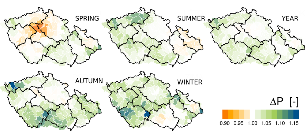
Fig. 3.3 Changes in precipitation from the 1961–1990 period to the 1980–2010 period for different seasons of the year.
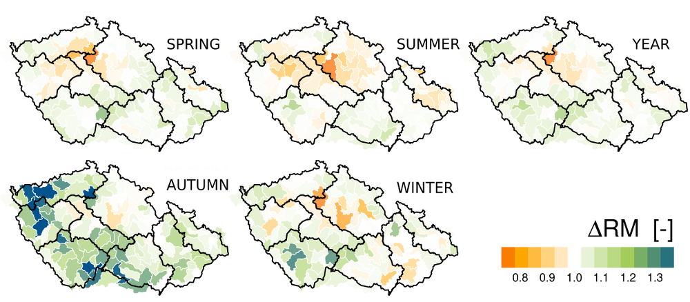
Fig.3.4 Changes of runoff (as estimated by a hydrological model) from the 1961–1990 period to the 1980–2010 period for different seasons of the year.
4 Climate change scenarios
To assess potential changes to the hydrological conditions expected to occur in Czech Republic’s catchments, two sets of climate change scenarios were considered apart from the observed changes; these were based on the ouputs of the ENSEMBLES and CMIP5 projects. At the same time, three representative simulations were chosen (from ENSEMBLES data) for the purpose of assessing the course to be taken by the possible implementations of the future hydrological conditions. These sets of scenarios are described in the following chapters.
4.1 Correction for systematic errors – ENSEMBLES data
Uring gridded observations of temperature and precipitation in the daily step, the simulations of regional climate models from Table 1.1 were corrected for systematic errors using the so-called quantile method (see e.g., Gudmundsson et al. (2012)). This (widely used) method has been chosen for the reason that, inter alia, simulations of the ALADIN-CLIMATE/CZ model corrected by this method have already been available. The method consissts in deriving a transfer function which guarantees that the values of the transformed series correspond to the same qualitles as the respective values of the original series. The period against which the simulations were corrected was chosen the same as in the ALADIN-CLIMATE/CZ case, i.e., 1961–1990. Formally the correction of the probability distribution of the simulated quantity \(P_m\) (e.g., of precipitation simulated by the climate model) using the distribution of the observed quantity \(P_O\) (e.g., the observed precipitation) can be written as the transformation
\[P_O = h(P_m)\](4.1)
The the transformed distribution \(h(P_m)\) is the same as that of the observed quantity. The transformation \(h\) is derived using the so-called probability integral transformation – which means making use of the fact that the distribution function of an arbitrary, continuous quantity has an uniform distribution. Then the transformation will take the form
\[P_O = F_O^{-1}[F_m(P_m)]\](4.2)
where \(F_m\) is an (empirical) distribution function obtained from simulated data for the control climate and \(F_O^{-1}\) is an emplirical quantile function derived from the observed series. In practical applications, this method often also entails the use of a statistical model of distribution of the given quantity (and the data are used solely to estimate the parameters of this distribution). Nonethless, in this project we stick to the empirical distribution and quantile function. In a simplified manner the procedure adopted can be described in such a way that the first step consists in ascertaining the probability of attaining the simulated precipitation and, subsequently, this is substituted by the value from the observed data which has the same probability. For the future climate it is sought to ascertain what are the probabilities of the quantities based on the distribution function for the control climate (\(F_m\)), whereupon the distribution function \(F_O^{-1}\) is used. As a rule the method is applied to individual months.
There are several pitfalls to be avoided when applying this method. In the case of precipitation the main concern is that the method cannot cope with the rectification of problems relating to the numbers of days with precipitation, or respectively, that it is unable to add more days in the case that the number of days with precpitation is low. Nonetheless, it is rather the opposite case which is typical of most climate models, i.e., that the number of days with precipitation is too high. Another problem connected with the corrections of both precipitation and temperature is that it it not clear how one could correct those values which are higher (or lower) than in the case of the simulation performed for the control climate. The approach usually considered here is linear ecxtrapolation of the highest values.
The Fig. 4.1 and Fig.4.2 show the original error of precipitation and temperature estimates and the error of corrected data. Generally, the summer precipitation values lend themselves better to simulation (their systematic error being as a rule within the range of −25%–25%) that those pertaining to the other seasons of the year (which are mostly overestimated by 30%–80%). The average error varies around approximately 30%. It is evident that generally, the correction procedure is rather successful in eliminating the systematic error associated with the various models. Simulations which significantly underestimate summertime precipitation and exhibit an excessive percentage of days free from rainfall are an exception (espcially HIR_ARP). Once we validate the corrective formulas for the 1981–2010 period, we find that the systematic error grows higher and yet remains relatively small when contrasted with the original simulation (mostly ±10%).
The summer temperature is overestimated by most of the RCMs (by up to 5°C – HIR_ARP again), whereas for the other seasons of the year the systematic error varies within ±1.5°C for most RCMs. The quantile method can be relied upon to eliminate these systematic errors (within the season or period for which it was employed), but still, when validated for the 1981–2010 period, the summer temperatures are subject to a systematic underestimation by ca. 1°C, indicating that the systematic error is not a steady-state phenomenon, or that in fact it may be influenced to quite a considerable degree by long-term climate variability. The nonsteady-state character of systematic errors has been mentioned e.g., by Reifen a Toumi (2009) and Ehret et al. (2012) or by Ehret et al. (2012), and yet the correction for systematic errors is a widely used technique.
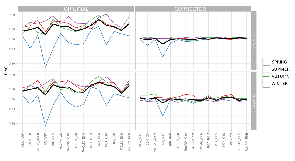
Obr.4.1 Systematic error (Czech Republic’s average) incurred by the average seasonal (color lines) and the annual (heavy solid line) precipitation for the original data and for corrected data contrasted with various observation periods.
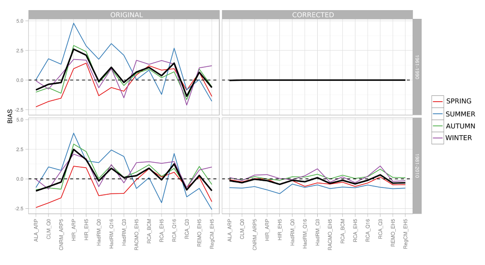
Obr.4.2 Systematic error (Czech Republic’s average) incurred by the average seasonal (color lines) and annual (heavy solid line) temperature for the original data and for corrected data contrasted with various observation periods.
The systematic error incurred in simulations of the maximim seasonal precipitation totals (i.e., total precipitation over a three-month period) is comparable with the error of the average total (Fig. 4.3). It is evident that the quantile method applied in the daily step cannot compensate for the systematic errors occurring in the values of the maximum seasonal totals. The reason is that the method does not take into account the persistence within the time series – i.e., in spite of the fact that the distribution of the daily values of the as-corrected simulation corresponds more or less rather accurately to the observed values; this does not apply to the distributions of the monthly, seasonal, and annual totals (and for the temperature averages – see Fig. 4.4). It is evident from the statistics of the corrected series shown in Fig. 4.3 (on top right) that the climate models underestimate the incidence of longer periods with rainfall, particularly in wintertime. Similarly, Fig. 4.4 indicates an excessive concentration of low-temperature days in summertime and of higher-temperature days in wintertime for approx. one half of the models.
An alternative, the treatment of which would however be outside the scope of this publication, is represented by the cascade correction (or incremental method) described e.g., by Haerter et al. (2011). The principle underlying this method is a gradual correction proceeding from long (for instance, seasonal) timescales to short (e.g., daily) timescales. Then the values submitted for correction as the deviations from the mean values of the higher time aggregations.
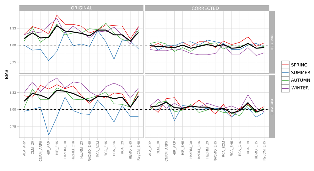
Fig.4.3 Systematic error (Czech Republic’s average) incurred by the maximum seasonal (color lines) and annual (heavy solid line) precipitation totals for the original data and for corrected data, contrasted with various observation periods.
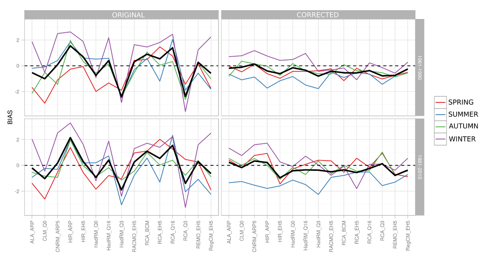
Fig.4.4 Systematic error (Czech Republic’s average) incurred by the maximum seasonal (color lines) and annual (heavy solid line) temperatures for the original data and for corrected data, contrasted with various observation periods.
4.2 Advanced incremental method – CMIP5 data
The generation of these scenarios made use of the data and R scripts provideed by the Royal Netherlands Meteorological Institute (KNMI), see Kraaijenbrink (2013), which lend themselves relatively easily to the application of the advanced incremental (ADC – Advanced Delta Change) method (Pelt et al. 2012) to any observed precipitation and temperature data in Europe. The advanced delta change method consists in transforming the observed series in such a way as to have the change between the transformed and the original time series correspond to the change in the climate model in-between the periods chosen. The simplest variant of this method will only transform the mean of the given quantity, and yet the analyses of the outputs of many climate models ave made it clear that the changes to the distributions, especially those of precipitation, become more comprehensive. The ADC method also allows to incorporate changes of variability in the transformation, which means that, in simplified terms, the extremes may be subject to changes different to those of the mean. When deriving the changes in precipitation from the climate model, the ADC method also takes the systematic errors of simulation into account. Inasmuch as the temperature is transformed linerarly the systematic error does not influence the resultant transformation of temperature.
Precpitation is transformed using the relation
\[ P^* = \begin{cases} a P ^ b & \text{pro $P^O < P^O_{90}$}\\ \frac{\bar{E}^F}{\bar{E}^C} (P^O - P^O_{90}) + a (P^O_{90})^b & \text{pro $P^O > P^O_{90}$}\end{cases} \](4.3)
where \(P^*\) are the transformed precipitation values, \(P\) is the observed precipitatin, \(P_{90}\) is the 90% quantile of precipitation, and the indices \(^O\), \(^C\) and \(^F\) indicate the observed data, the GCM data for the control period and those for the scenario period,\(a\) and \(b\) are the transformation parameters derived for 5-day blocks which guarantees the seasonal variability of the changes. Linear transformation for the values above \(P^O_{90}\) prevents any incidence of values that would be unrealistically high; at a relatively high frequency such values are the result of nonlinear transformations for \(P > P_{90}\) a \(b>1\).
The above-threshold value \(E = P - P_{90}\) is calculated for precipitation values higher than the 90% quantile of precipitation. The average above-threshold values in the GCM for the control and scenario periods are computed using the formula
\[\bar{E}^C = \frac{\sum P^C - P^C_{90}}{n^C} \quad \mathrm{a} \quad \bar{E}^F = \frac{\sum P^F - P^F_{90}}{n^F}\](4.4)
where \(n^C\) and \(n^F\) are the numbers of above-threshold values during the control and the scenario period, respectively. The transformation parameters \(a\) and \(b\) are derived from the values of the 60% (\(P_{60}\)) and 90% (\(P_{90}\)) quantiles of precipitation using
\[b = \frac{\log[g_2 P^F_{90}/ (g_1 P^F_{60})] }{\log[g_2 P^C_{90}/ (g_1 P^C_{60})]}\\ a = P^F_{60}/(P^C_{60})^b g_1^{1-b}\](4.5)
where \(g_1\) and \(g_2\) are correction factors expressing the systematic errors incurred in \(P_{60}\) and \(P_{90}\) in the GCM simulation performed for the control period.
\[g_1 = P^O_{60}/P^C_{60}\] \[g_2 = P^O_{90}/P^C_{90}\](4.6)
nasmuch as the values \(P_{60}\), \(P_{90}\), \(\bar{E}^C\) and \(\bar{E}^F\) re relatively variable in time, the average monthly values of these quantities are smoothened by a weighted moving average using the weights of 0.25, 0.5 a 0.25. Simultaneously, the value of the parameter \(b\) and of the ratio \({\bar{E}^F}/{\bar{E}^C}\) exhibits a considerable spatial variability. Therefore, these parameters are averaged in a spatial moving window, from a regular neighborhood of 8 grid boxes.
The parameters \(a\) and \(b\) available were derived for the whole of Europe (Kraaijenbrink 2013), with the systematic errors computed based on a gridded E-OBS data set (Haylock et al. 2008), aggregated to the climate model resolution (i.e., ca. 150 × 120 km, ca. 5 grid boxes relevant for the Czech Republic, where E-OBS employs a resolution of 25 × 25 km). It is well known that the E-OBS is of different quality for different parts of Europe and that the Czech Republic ranks among countries with a relatively low density of data serving the generation of the E-OBS data set. All the same, we assume that any systematic error introduced by the use of E-OBS data is negligible compared to the typical systematic errors incurred by the climate models, also bearing in mind the size of the GCM grid box to which the data are aggegated.
With the ADC method, the transformation of temperature is performed as follows:
\[T^* = \frac{\sigma^F}{\sigma^C} (T - \bar{T}^O) + \bar{T}^O + \bar{T}^F -\bar{T}^C\](4.7)
where \(T^*\) is the transformed temperature, \(\bar{T}^O\), \(\bar{T}^C\) and \(\bar{T}^F\) are the transformed average monthly temperatures for the observed data, GCM is the control and scenario period, and \(\sigma^C\) and \(\sigma^F\) are the standard deviations of daily temperatre for the control and the scenario periods in the GCM.
The parameters derived for GCM from Table 1.2 were subsequently used to transform the gridded precipitation and temperature (Štěpánek et al. 2011) originating fro the CHMI (cf. Chapter 1.1); for the sake of consistency with GCM data, only the 1961–1995 period was considered. Obviously, these data could also be theoretically used to correct the systematic errors incurred in deriving the transformation parameters for precipitation, but this would amount to repeating the entire derivation process and was not possible for time constraint reasons
Fig. 4.5 indicates the course followed by the transformation parameters \(a\), \(b\) and \(\bar{E}^F\) and \(\bar{E}^C\) for various RCP scenarios and time periods. The parameter a impacts the mean precipitation. Its values indicate that what mainly occurs in the simulations is the increase of precipitation during the period from approx. November until April/May and a reduction for the remainder of the year. Simulataneously, trhe increasing variability of summertime precipitation (parameter b) as well as of the share of daily totals higher than the 90% quantile can be seen.
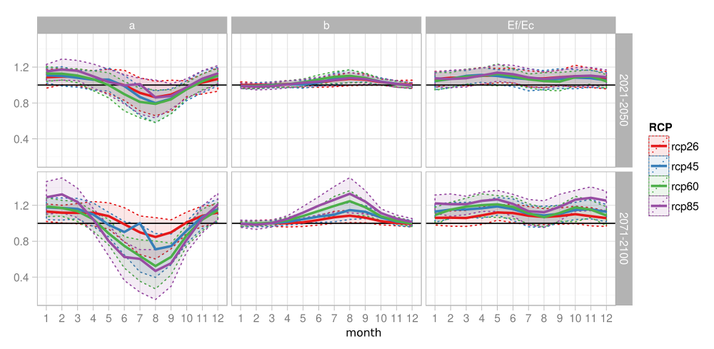
Obr.4.5.Seasonal variation of the transformation parameters of Equation 4.3 amd varopis RCL scenarios and time periods. The heavy line depicts the median of the GCM simulations for the given RCP scenario, the inter-quartile spans are shown in color.
5 Application of the scenarios and an overview of impacts
For hydrological modeling, two climate change scenarios differing in nature were available in addition to the observed data:
- For hydrological modeling, two climate change scenarios differing in nature were available in addition to the observed data:
- the observed time series transformed using the ADC method on the basis changes occurring betweem the scenario periods of 2021–2050 and 2071–2100 and the control period 1961–1995 for 191 simulations from the CMIP5 project
These scenario series were used in the hydrological balance simulations performed by the Bilan model using the parameters described in Chapter 2. Inasmuch as the matter of primary interest has been to derive the changes occuring to the elements of the hydrological balance rather then their absolute values for the different years under scrutiny, we have further on used the monthly, seasonal, and annual changes of selected elements. The period 1981–2010 was chosen as the reference period for the changes, because on the one hand it is more representative of the prevailing hydroclimatic conditions and, on the other hand, this also is the period previously used in the IPCC Fifth assessment report (Stocker et al. 2013). Subsequently, for the ENSEMBLES simulations, the changes of the average values between the periods 1961–1990, 1971–2000, … 2071–2100 and the 1981–2010 period were computed. Further on the periods are also designated by their centers, i.e., 1975, 1985, … 2085 and the control period 1995. Owing to the fact that for the CMIP5 scenarios the only changes available were those from the 2035 and 2085 periods referred to the 1975 period, it was assumed for the purpose of deriving the changes for the lacking thirty-year period that the course followed by the 30-year averages in-between the available averages (1975, 2035, and 2085) is influenced by the effects of radiation rather than by the natural variability, and that it is therefore possible to fit a smooth curve on the data for these periods and from this to estinate the changes for all the other periods. For every GCM model, RCP concentration scenario and month, the values of the averages (for runoff, precipitation, temperature) were interpolated using a third-power spline function. Suseqently, the changes were computed in analogy to the case involving ENSEMBLES dat.
6 Overview of impacts
At this point we shall concentrate on presenting the body of results obtained and some statements relative to the average changes of the quantities selected, rather than on a detailed discussion of impacts. The results are presented in the subsequent sections of the website.
A basic overview of the modeled climate change impacts in the Czech Republic is given in Fig. 6.1. From the point of view of the historical context of modeling the climate change in the Czech Republic these (average) results are in no way surprising. In agreement with earlier published results, there occurs an increase in runoff from the catchments in wintertime, due in part by enhanced wintertime precipitation and in part by an earlier onset of the period of thaw, or possibly by limited snow cover caused by warming. It is rather a reduction of both total runoff and base flow during the other months. This is attributed to a higher evapotranspiration (being a consequence of increased temperature) which is no longer adequately compensated by increased precipitation. On the top of this, for the concentration scenarios RCP6.0 and RCP8.5 there also occurs a reduction in summertime precipitation. The average scope of changes for the set of simulations considered is also shown in Table 6.1. The average changes were computed in such a was that the Czech Repblic average fwas established in the first step for each cimate model simulation, whereupon these averages were used to compute te average changes applicable to the differen scenarios of emissions/concentrations, which means that the spans were computed rom five values – i.e., 4 RCP + 1 SRES scenario. The number of elements considered in computing the averages is different for different scenarios: 1950 A1B, 5850 RCP2.6, 7020 RCP4.5, 3770 RCP6.0, 8190 RCP8.5. Clearly, in individual cases (for specific catchments and climate model simulations) the values of the changes incurred may be significantly outside the scope of the values shown in Table 6.1. For the sake of interest, let us consider the over-all scopes of changes for all the chatchments and simulations as shown in Table 6.2. It is one of the simplest ways of how to express the uncertainty inherent to the set of models where however the scope is substantially overestimated – for example, a 20-fold increase of wintertime base flow can be regarded as unrealistic.
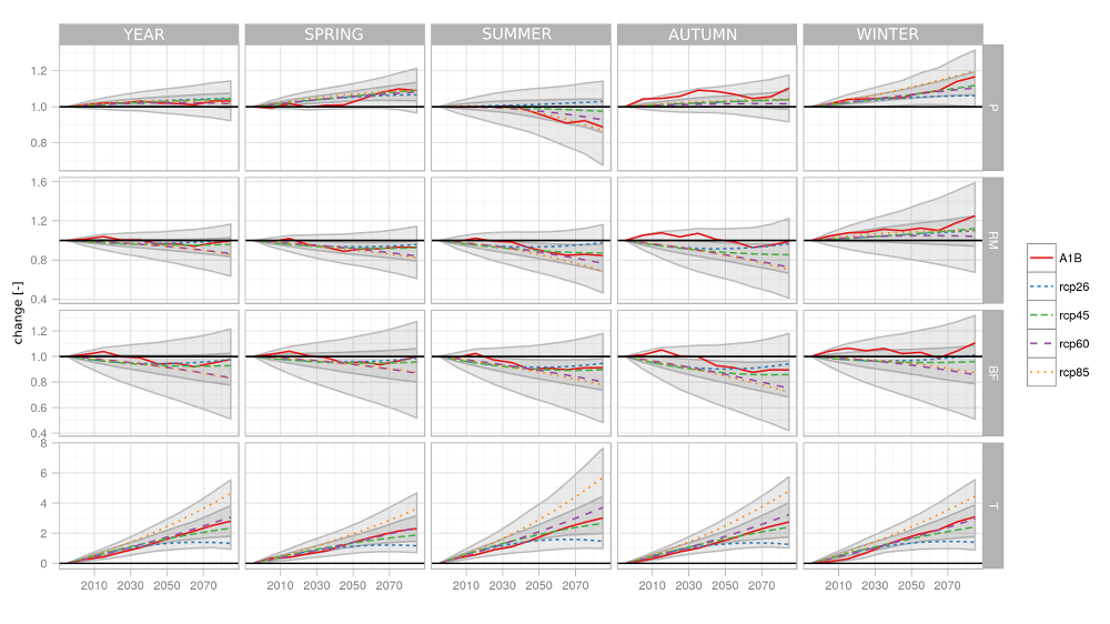
Fig. 6.1 Changes of precipitation (P), total model runoff (RM), model base flow (BF), and temperature (T) for various time horizons and emission/concentration scenarios (color lines). Areas enclosing 90 % and 75 % of all projections are depicted by gray polygons. The are average values for the Czech Republic
Table 6.1 Extent of average changes as per the various concentration scenarios for different seasons of the year, time horizons, and quantities.
| YEAR | SPRING | SUMMER | AUTUMN | WINTER | |
|---|---|---|---|---|---|
| 2011–2040 | |||||
| P | 1.02 - 1.03 | 1.00 - 1.04 | 1.00 - 1.01 | 1.01 - 1.06 | 1.03 - 1.05 |
| RM | 0.97 - 1.01 | 0.95 - 0.96 | 0.93 - 0.99 | 0.92 - 1.04 | 1.03 - 1.08 |
| BF | 0.95 - 1.00 | 0.96 - 1.01 | 0.93 - 0.97 | 0.91 - 1.00 | 0.97 - 1.04 |
| T | 0.74 - 1.18 | 0.63 - 0.97 | 0.89 - 1.36 | 0.76 - 1.19 | 0.68 - 1.19 |
| 2041–2070 | |||||
| P | 1.02 - 1.04 | 1.04 - 1.07 | 0.94 - 1.02 | 1.02 - 1.07 | 1.05 - 1.12 |
| RM | 0.93 - 0.97 | 0.89 - 0.94 | 0.84 - 0.94 | 0.83 - 0.99 | 1.05 - 1.13 |
| BF | 0.90 - 0.95 | 0.93 - 0.96 | 0.86 - 0.92 | 0.83 - 0.91 | 0.92 - 1.03 |
| T | 1.36 - 2.72 | 1.17 - 2.17 | 1.56 - 3.26 | 1.33 - 2.78 | 1.40 - 2.68 |
| 2071–2100 | |||||
| P | 1.02 - 1.05 | 1.07 - 1.09 | 0.87 - 1.03 | 1.02 - 1.10 | 1.06 - 1.20 |
| RM | 0.86 - 1.00 | 0.82 - 0.96 | 0.69 - 0.98 | 0.70 - 0.99 | 1.04 - 1.25 |
| BF | 0.83 - 0.98 | 0.87 - 1.00 | 0.78 - 0.95 | 0.72 - 0.94 | 0.86 - 1.11 |
| T | 1.33 - 4.64 | 1.17 - 3.62 | 1.47 - 5.70 | 1.27 - 4.80 | 1.40 - 4.46 |
Table 6.2 Extent of average changes deriving from different simulations and catchments, for different seasons of the year, time horizons, and quantities.
| YEAR | SPRING | SUMMER | AUTUMN | WINTER | |
|---|---|---|---|---|---|
| 2011–2040 | |||||
| P | 0.93 - 1.16 | 0.81 - 1.26 | 0.79 - 1.31 | 0.87 - 1.33 | 0.76 - 1.28 |
| RM | 0.57 - 1.73 | 0.51 - 1.67 | 0.51 - 1.96 | 0.25 - 4.60 | 0.39 - 2.57 |
| BF | 0.44 - 2.35 | 0.42 - 2.07 | 0.25 - 3.47 | 0.07 - 9.69 | 0.32 - 5.62 |
| T | 0.18 - 1.99 | -0.28 - 2.00 | 0.07 - 2.62 | 0.01 - 1.74 | -0.16 - 2.14 |
| 2041–2070 | |||||
| P | 0.80 - 1.22 | 0.8.5 - 1.37 | 0.60 - 1.28 | 0.78 - 1.39 | 0.70 - 1.35 |
| RM | 0.29 - 2.07 | 0.37 - 1.97 | 0.24 - 1.86 | -0.06 - 5.29 | 0.17 - 2.75 |
| BF | 0.13 - 2.37 | 0.17 - 2.13 | 0.11 - 3.29 | -0.10 - 5.40 | 0.01 - 9.07 |
| T | 0.35 - 4.17 | 0.30 - 3.57 | 0.36 - 5.67 | 0.28 - 3.82 | 0.38 - 4.18 |
| 2071–2100 | |||||
| P | 0.74 - 1.29 | 0.78 - 1.48 | 0.51 - 1.38 | 0.74 - 1.49 | 0.87 - 1.61 |
| RM | 0.20 - 2.38 | 0.24 - 4.58 | 0.16 - 2.34 | 0.02 - 4.89 | 0.09 - 5.37 |
| BF | 0.10 - 3.66 | 0.10 - 2.99 | 0.05 - 3.24 | 0.01 - 7.59 | 0.01 - 18.83 |
| T | 0.16 - 6.71 | 0.13 - 5.86 | -0.03 - 9.28 | -0.32 - 6.87 | 0.30 - 6.80 |
7 References
BERAN, A, M PELÁKOVÁ, L KAŠPÁREK, M HANEL a R KOŽÍN, 2014. Výpočet velikosti dotace podzemních vod za pomoci hydrologického modelování na vybraných hydrogeologických rajonech ČR. VTEI. roč. 56, č. 4.
BERAN, A., S. HORÁČEK a M. HANEL, 2011. Zjednodušení metody výpočtu potenciální evapotranspirace v nové verzi modelu BILAN. VTEI. roč. 53, č. mimořádné číslo III, s. 15–18.
COLLINS, Matthew, Ben BOOTH, Glen HARRIS, James MURPHY, David SEXTON a Mark WEBB, 2006. Towards quantifying uncertainty in transient climate change. Climate Dynamics. B.m.: Springer Berlin / Heidelberg, roč. 27, č. 2, s. 127–147.
EHRET, U, E ZEHE, V WULFMEYER, K WARRACH-SAGI a J LIEBERT, 2012. HESS Opinions„ Should we apply bias correction to global and regional climate model data?" Hydrology and Earth System Sciences Discussions. B.m.: Copernicus GmbH, roč. 9, č. 4, s. 5355–5387.
GUDMUNDSSON, L, JB BREMNES, JE HAUGEN a T ENGEN-SKAUGEN, 2012. Technical Note: Downscaling RCM precipitation to the station scale using statistical transformations–a comparison of methods. Hydrology and Earth System Sciences. B.m.: Copernicus GmbH, roč. 16, č. 9, s. 3383–3390.
HAERTER, JO, S HAGEMANN, C MOSELEY a C PIANI, 2011. Climate model bias correction and the role of timescales. Hydrology and Earth System Sciences. B.m.: Copernicus GmbH, roč. 15, č. 3, s. 1065–1079.
HAYLOCK, M, N HOFSTRA a A KLEIN-TANK, 2008. A European daily high-resolution gridded data set of surface temperature and precipitation for 1950–2006. Journal of Geophysical Research. roč. 113, č. D20, s. D20119.
HEWITT, C. D. a D. J. GRIGGS, 2004. Ensembles-based Predictions of Climate Changes and their Impacts. Eos. roč. 85, č., s. 566.
HORÁČEK, S., O. RAKOVEC, L. KAŠPÁREK a A. VIZINA, 2009. Vývoj modelu hydrologické bilance BILAN. VTEI. roč. 51, č. mimořádné číslo I, s. 2–5.
KAŠPÁREK, L, 1989. Odhad směrodatné chyby průtoků a jejich základních charakteristik. B.m.: Český hydrometeorologický ústav.
KAŠPÁREK, L, JV DATEL, M HANEL, A HRABÁNKOVÁ a M KNĚŽEK, 2012. Rebilance zásob podzemních vod: Metodika stanovení průměrné hodnoty přírodních zdrojů podzemních vod kvartérních hydrogeologických rajonů. B.m.: Výzkumný ústav vodohospodářský T. G. Masaryka, v.v.i.
KAŠPÁREK, L, R NAAROVÁ a Špalle M, 2000. Hodnocení a modelování srážko-odtokových vlastností povodí. B.m.: Výzkumný ústav vodohospodářský T. G. Masaryka, v.v.i.
KRAAIJENBRINK, Philip, 2013. Advanced Delta Change method. B.m.: KNMI.
KRÁSNÝ, J, M KNĚŽEK, A ŠUBOVÁ, H DAŇKOVÁ, M MATUŠKA a V HANZEL, 1982. Odtok podzemní vody na území Československa. Praha: ČMÚ v SNTL.
MÁCA, P, S HORÁČEK a A VIZINA, 2013. Optimalizace parametrů modelu Bilan metodou SCDE. 2013.
OUDIN, Ludovic, Lætitia MOULIN, Hocine BENDJOUDI a Pierre RIBSTEIN, 2010. Estimating potential evapotranspiration without continuous daily data: possible errors and impact on water balance simulations. Hydrological Sciences Journal. roč. 55, č. 2, s. 209–222.
PELT, S. J. van, J. BEERSMA a T. A. BUISHAND, 2012. Future changes in extreme precipitation in the Rhine basin based on global and regional climate model simulations. Hydrology and Earth System Sciences. roč. 16, č., s. 4517–4530.
REIFEN, C. a R. TOUMI, 2009. Climate projections: Past performance no guarantee of future skill? Geophys. Res. Lett. roč. 36, č. L13704.
STOCKER, Thomas F, Dahe QIN, Gian-Kasper PLATTNER, M TIGNOR, Simon K ALLEN, Judith BOSCHUNG, Alexander NAUELS, Yu XIA, Vincent BEX a Pauline M MIDGLEY, 2013. Climate change 2013: The physical science basis. B.m.: Intergovernmental Panel on Climate Change, Working Group I Contribution to the IPCC Fifth Assessment Report (AR5)(Cambridge Univ Press, New York).
ŠTĚPÁNEK, P, P ZAHRADNÍČEK a R HUTH, 2011. Interpolation techniques used for data quality control and calculation of technical series: an example of a Central European daily time series. IDÖJÁRÁS - Quarterly Journal of the Hungarian Meteorological Service. roč. 115, č. 1–2, s. 87–98.
Climate change impacts on the hydrological situation in the catchments of the Czech Republic
Set of specialized maps
Martin Hanel, Stanislav Horáček, Ondřej Ledvinka, Martin Tomek, Radim Tolasz, Martin Stříž, Jan Daňhelka, Kateřina Hánová
The set of maps shown represents the estimates of potential changes in seasonal and annual averages of the hydrometeorological variables caused by climate change for 130 catchments covering Czech Republic’s territory, also synthesizing the simulated changes based on an extensive set of (ca. 200) climatic model simulations, including those simulations that served for the preparation of source data for the Fifth Assessment Report of the Intergovernmental Panel on Climate Change (IPPC AR5), the so-called CMIP5 set of models. The maps illustrate the changes in precipitation (P), temperature (T), potential evapotranspiration (PET), basin evaporation (E), total runoff (RM), baseflow (BF), the 95% quantile from the line of exceeding the monthly total runoff (RM95) and the baseflow (BF95), and the baseflow index (i.e., the baseflow to total runoff ratio, BFI).
In terms of its area coverage and time span as well as in terms of the number and up-to-dateness of the modeled climate change scenarios and of easy access thanks to a web application, this set of maps is unique in the Czech Republic and as such may find a wide range of applications relating to long-term planning of water resources, land use, the energy sector, etc.
The set of maps serves as an indicator of (spatially) averaged changes for the various catchments of the defined set (as entities). While for precipitation and temperature it is not necessary, owing to the over-all uncertainty of estimates, to consider the spatial variability of the changes within the framework of these catchments, in the case of the hydrological variables the estimated changes cannot simply be expected to be evenly distributed among the various subcatchments. Here the results have to be interpreted making use of the knowledge of the local hydrological conditions as well as of current trends and potential problems.
Estimates of the character of the future climate suffer from considerable uncertainty stemming from the chancy socio-economic development of society, an insufficient capacity for modeling the climate, and the inherent variability of the climate-related variables. This is why the maps presented here do not indicate a single change value in the case of one variable for one catchment, time horizon, and season of the year, but rather show a range of changes for various models and scenarios.
The set of maps was developed within the research project TA02020320 Support of long-term planning and design of adaptive measures in the area of water management within the climate change context co-funded by the Technology Agency of the Czech Republic.